
Transdimensional Inversion ( AGU 2014 Poster, Earth Scope 2015 Poster )
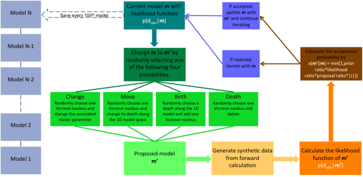
Most inverse problems in the geosciences treat the number of unknowns (or model parameters), k, as a constant. Transdimensional inversion is the name given to the case where this assumption is relaxed, and k is treated as an unknown (Sambridge et al., 2013). While allowing an adaptive parameterization, it provides a parsimonious solution that fully quantifies the degree of knowledge one has about seismic structure. Transdimensional inversion is also an approach based on a Bayesian framework using partition modeling, which means all information is represented in probabilistic terms and the aim of inversion is to recover the model probability given the observed data. The figure above shows an overview of the reversible-jump Markov chain Monte Carlo algorithm we used for transdimensional inversion. I'm currently working on synthetic test of joint inversion including surface wave dispersion, H/Z ratio, and receiver function.
Lithospheric structure of mid-ocean ridge Click to View Our AGU Poster
Undergraduate Research Project. Advisor: Prof. Huajian Yao
Research Summary
The time derivative of the long-time cross-correlation of ambient seismic noise can be used to estimate the Empirical Green’s functions (EGFs) between pairs of seismographs. These EGFs reveal velocity dispersion at relatively short periods, which can be used to resolve structures in the crust and uppermost mantle better than with traditional surface-wave tomography. In this research, we use the seismic surface-wave data recorded by 28 OBSs at the QDG transform fault system to measure the Rayleigh-wave dispersion curves using two-station analysis. By combining the Rayleigh-wave dispersion curves from EGFs and traditional two-station analysis, we could perform a shear velocity structure inversion to constrain the lithosphere structure beneath the equatorial eastern Pacific Ocean.
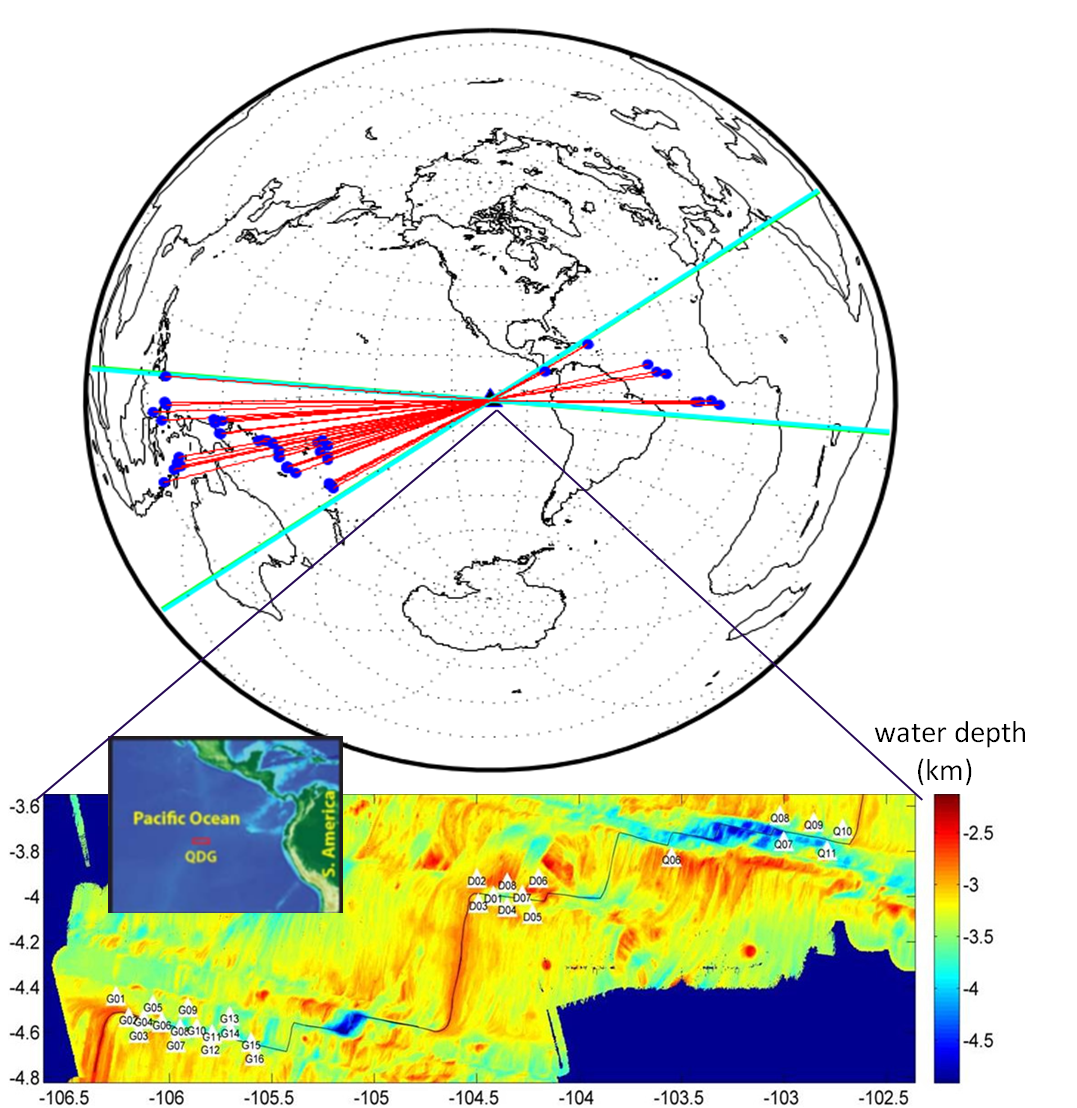
Selected earthquake events
and location of 28 broadband OBSs
|
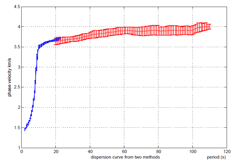
Dispersion curves from ambient noise(blue) and earthquake surface wave(red)
|
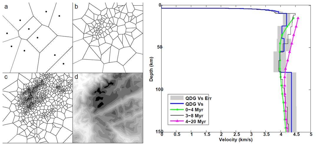
Structure inversion using neighbourhood algorithm(left) 1-D average velocity structure(rigth)
Conclusion:
Our final model shows a 80km deep low velocity zone in the upper mantle beneath the mid-ocean ridge area. This low velocity zone indicates a very young seafloor age which meets the characteristics of the mid-ocean ridge region. Further work will be done on the aspect of the radial anisotropy from inversion of both Rayleigh and Love waves, and we can constrain the upper mantle deformation due to upwelling of the hot asthenospheric material better.
Our final model shows a 80km deep low velocity zone in the upper mantle beneath the mid-ocean ridge area. This low velocity zone indicates a very young seafloor age which meets the characteristics of the mid-ocean ridge region. Further work will be done on the aspect of the radial anisotropy from inversion of both Rayleigh and Love waves, and we can constrain the upper mantle deformation due to upwelling of the hot asthenospheric material better.
Sea ice influence on microseism
National Undergraduate Innovation Program. Advisor: Prof. Sidao Ni
Research Summary
As we all know, Arctic area is one of the most important spots for researching. We tried to explore the relationship between the sea ice seasonal variability on the Arctic Ocean and the microseism. Although there's some related researches in the Antarctic, it's harder to reach the same conclusion because of the complex source of microseism, which is generally believed to be the oceanic storm.To solve this problem, we came to a solution by comparing the amplitudes of the microseism at different latitudes. In this way, the noise spectrograms seen at lower latitudes are typical of seasonal ocean microseism variability and we could see the influence of sea ice at higher latidudes.
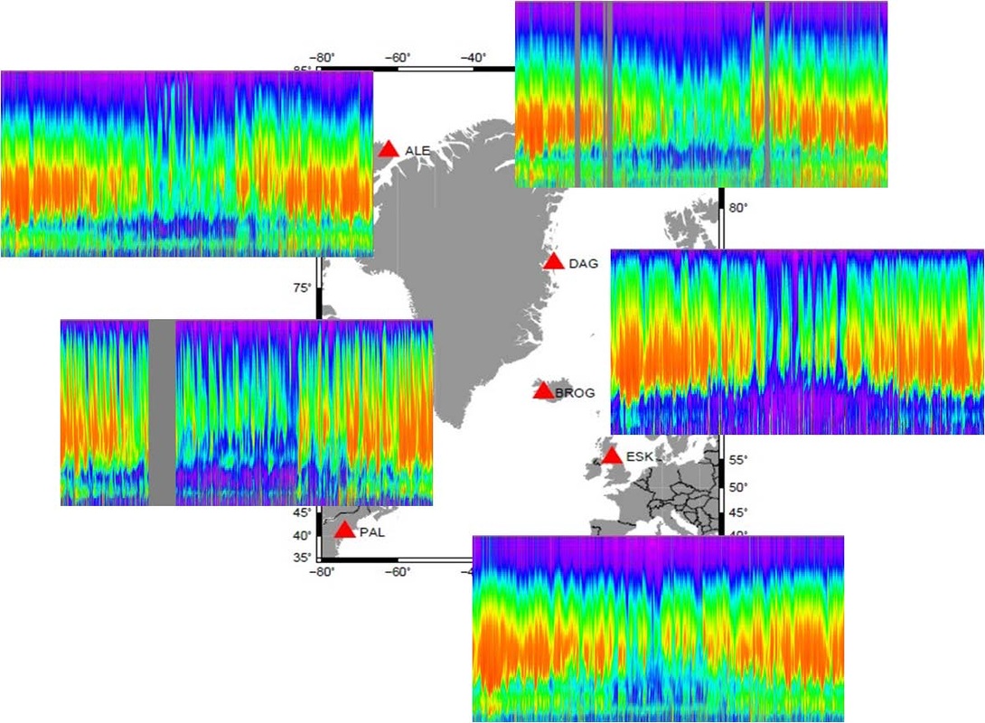
Yearly noise spectrograms at different latitudes
|
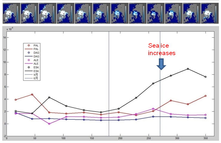
The amplitudes at higher latitude are hampered because of the sea ice
|
Conclusion:
Through the noise spectrograms, we can see that the amplitudes of microseism at higher latitude were hampered by the increasing area of sea ice. This result can be seen more clearly at a specific frequency of 0.30Hz, which is compatible with the theory of "double-frequency".
Through the noise spectrograms, we can see that the amplitudes of microseism at higher latitude were hampered by the increasing area of sea ice. This result can be seen more clearly at a specific frequency of 0.30Hz, which is compatible with the theory of "double-frequency".
